Big Theorems of Differential Calculus

I packaged the four big theorems of continuity and differentiation into one 40 minute lesson today.  The goal was to present and explain the Intermediate Value Theorem (IVT), the Extreme Value Theorem (EVT), Rolle’s Theorem (RT), and the Mean Value Theorem (MVT).  We had just finished a lesson on finding extreme values of functions over closed intervals.  Acting on a teaching tip from my colleague, I sought to convince the students informally that the opposite of each statement would be impossible.

I’ve struggled with how to present these results in Calculus classes over the years.  In an honors Calculus course, where we deduced each result of Calculus carefully from the axioms of the real numbers, I’ve gone through the proofs in detail.  For example, I’ve deduced the IVT from the definition of continuity and the completeness axiom using the method of successive bisection.  In Calculus for Life Science or Calculus for Business, I’ve settled with drawing the graphs of several continuous functions over closed intervals and verifying the claim of the IVT in each case with the students.  For Analytic Geometry and Calculus I, I needed to find a happy medium between these approaches.  The full argument, presented with less notation, would still involve too much generality and require erecting a lot of scaffolding earlier in the term.  The “proof by example” method always leaves the lesson feeling hollow, because of the natural student response of, “Yeah, but what’s the point?”

This time, I might have found the right balance.  Before stating the theorems, I set up my sonic range finder at the front of the room, projected the logging software on the screen at the front, and asked for a student volunteer.  I placed index cards on the floor marking a distance of 1 m from the detector and a distance of 3 m from the detector.  Then I issued the student the following challenge:

• Your challenge is to start 1 m from the detector and end 3 m from the detector at 5 sec and move in such a way that your graph does not cross the horizontal line at distance equals 2.  You can move towards and away from the detector in any way you want, but you can’t move out of the beam.

I gave the student 20 seconds or so to think of a plan of action, and then they gave it a try.  Of course, the task is impossible by the IVT because their position varies continuously with time over the closed interval [0,5], but that didn’t stop the student from trying much to the entertainment of their classmates.  One student tried moving almost to 2m then jumping above the beam over the 2 m mark and continuing to three.  A valiant effort, but this would have required a vertical leap exceeding that of an all star NBA guard, so the effort predictably failed.  But it made the point very real.  To get from 1 m away to 3 m away, one must go through 2 m.  In fact, one must visit every intermediate distance between 1 m and 3 m, not just 2 m.  This is the IVT.

With a different volunteer, I issued this directive:

• Your challenge is to start at 1 m from the detector and end at 1 m from the detector but never have the slope of your graph be zero.  You can move towards and away from the detector in any way you want, but you can’t move out of the beam.

For one volunteer, this prompted a question, “Could I just stand here at 1 m away for the whole time?”  I responded with “Well, let’s see” and started collecting data from where he stood at the 1 m mark.  A horizontal line graph was produced and he was able to answer his own question.  I gave him 20 more seconds to develop a strategy and then he gave it another try.  Interestingly, he tried moving slowly towards the detector to produce negative slope, then realized half way that he needed to turn around and laughed out loud when his distance versus time graph developed a slope of zero when he had stopped.  I confessed again that this is an impossible task because his distance from the detector was varying continuously over [0,5] and was differentiable (because we can make sense of his instantaneous velocity) over (0,5) and f(0)=f(5).  Thus, the derivative had to be zero at some point in (0,5) by Rolle’s Theorem.

The class was in to the lesson by this point, with neighboring students arguing about whether they could or could not meet the challenge by doing something different and realizing that doing so would be impossible.  For the last challenge, I found one more volunteer and said:

• Okay, you have the toughest challenge.  You are going to start 1 m away from the detector and end 3 m from the detector after 5 seconds, moving however you wish in the mean time (towards or away from the detector, staying within the beam).  Your position will change 2 m over 5 seconds, so your average velocity will be 2/5 m/sec.  Your challenge is to complete this motion without having your instantaneous velocity be 2/5 m/sec at some time during your movement.  If you were to walk steadily from 1 m to 3 m over 0 sec to 5 sec, your graph will be linear with slope 2/5 m/sec, so don’t do that.

The ideas the volunteers displayed were wonderful.  One student tried to rapidly travel towards 3 m, overshoot, and then back up.  The other volunteer in the other section choose to wait at 1 m for 3 seconds, then rapidly move to 3 m.  I asked the class to vote whether the volunteer had succeeded, and then led a whole class discussion analyzing their graph to see why they failed.  Of course, this is impossible by the Mean Value Theorem.

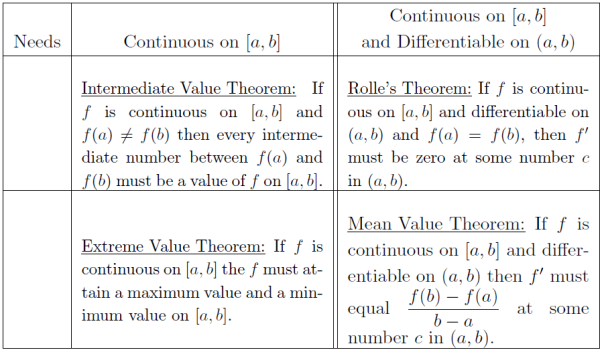
I wrote the four theorem statements on the board, organized in a table.

At this point, they were ready to understand the general statements because thinking through the challenges helped them understand that what matters is not what the function is, but what properties it has and what we assumed about it.  The generality was less mystifying because instead of analyzing examples, they had tried to create a function which met the challenge.  Each theorem says that something must happen. Having the conclusion not happen is impossible.

I followed this discussion with two ConcepTests to see if they could transfer the ideas to another setting.  For the first one, there was broad consensus on A and B.

Discussing it with the class, I emphasized how the rider’s velocity would likely be slower than the average when plodding uphill, faster than the average when racing downhill, but by the MVT had to equal the average velocity at some point.

For the second question, the first vote was split and, while they had a lot to say with their neighbors, the discussion changed some minds to B but not to C.

I couldn’t tell what drew most of them to B but I suspect that at least some had confused equality of at some and the average rate of change with the intersection of the curve with the dashed line.  Leading the class, I talked through the picture emphasizing that the average rate of change computes the slope of the dashed line, while computes the slope of the tangent line to the curve at .  Using my pen as a segment of the tangent line, I followed the graph from one end to the other and we identified the three places where the slopes were the same.  Working through this question emphasized that the MVT says it must happen that the slope of the curve at some point agrees with the slope of the secant line between the endpoints, but says nothing about how often this happens or where.  Just that it must happen.  The four big theorems of differential calculus explain what must happen for any function on a closed interval, under certain hypotheses.

Physical or Digital?

With the 4th of July falling on a Thursday this year, one of my summer Calculus courses ended up a day short.  In order to keep the Monday-Wednesday course on the same schedule, I decided to make Wednesday the 3rd into an extra activity day.  In the first hour, we did a class activity using a sonic range finder (motion detector) which I’ve done before.  I give the students a worksheet with eight verbal descriptions of motion back and forth along a straight line and ask them to sketch a graph of each motion, plotting distance from the detector vs. time.  The students are divided into groups for discussion of their graphs and then, one-by-one, I have each group come up and demonstrated one of the motions in front of the detector.  The data logging software that comes with the device plots the graph of their motion in real time and I display it for the whole class on the projector.  We discuss the nature of the graph at various points during each motion and plant the seeds for further understanding when we later talk about derivatives.

For the second hour, I thought it would be good to put our heads together on an interesting analytic geometry problem.  At this point in this summer course though, we had barely talked about limits.  In fact, our analysis of limits to that point only involved making numerical tables and looking at graphs to analyze trends.  So we didn’t have much to work with.  Here is the problem (from Stewart’s Problems Plus).

Let P be a point on the parabola different from the origin O.  The perpendicular bisector to OP intersects the -axis at a point Q.  Do the positions of the points Q have a limit as P approaches the origin?

This can be answered by finding an equation for the perpendicular bisector and determining its -intercept Q as a formula in the -coordinate of P, then taking the limit as .  But what I wanted the students to do was to do the geometric experiment of constructing the points Q for a family of points P along the parabola and looking to see if their locations showed a trend (just as we had done with numerical tables for limits of functions before).

Now, doing this properly requires some equipment.  First of all you need an accurate representation of the standard parabola on a Cartesian coordinate grid.  If you plot one by hand, your tick marks on the horizontal and vertical axes are likely to be slightly uneven and your axes may not be perfectly perpendicular, not to mention the fact that your curve is unlikely to be perfect parabola.  Any one of these small errors will destroy the geometry of the problem and the experiment will not yield the desired result.  So I created such a plot using FooPlot, imaging in the window [-1,1] x [-0.2,1.2], printed and distributed one to each student.  Knocking on doors around the department, I dug up a class set of rulers for the students to use but was unable to locate some compasses.  That’s okay, I thought, they could measure to find the midpoint.  Furthermore, the rulers are clear and they could just overlay and align a measurement mark on the ruler with the line OP at the midpoint to get a pretty good approximation to the perpendicular bisector of OP.  This would enable them  to plot Q and quickly move on to repeat the process with a new point P closer to O on the parabola.

Unfortunately, this did not go as smoothly as I thought it would.  There were confusions about measuring techniques with rulers and the meaning of the phrase perpendicular bisector.  Even we they got most of the steps, the technique of aligning a measuring mark with OP to produce a perpendicular line was susceptible to amplification of error.  When you don’t get the angle of the bisector exactly at 90 degrees, even a small error in angle translates into a wide error in the position of the point Q.  Not only did it take much longer than I anticipated, because I had to run around giving mini-lessons in geometry, but the error rate was so high, that most of the students didn’t see the trend in positions emerge.

So, I need to re-tool this project.  But what should I do?  Seriously, I need some ideas here.  After careful reflection, I called into question my assumptions of their background skills.  It’s easy to rant about “Kids these days!” and what they “should have learned before…” but that’s really just venting frustration.  I was frustrated because the goal of my activity was compromised because of the mismatch of my expectations and their skills.  Perhaps they would have seen the pattern emerge if I took the construction out of their hands and had them do it on the computer?  We could have gone into the computer lab and used GeoGebra to carry out the construction with a moving point (rather than a smaller discrete family) with perfect precision.  Some would argue that I would be missing the opportunity to develop their spatial reasoning skills by converting to the digital version, but I’m not so sure that’s true.  Yes, I would not be developing their art skills of using a ruler, but would the software not give them the same, if not better, visualization?  Ultimately, the development of that visualization is what I really want, right?

I’ve never included a poll of readers here before, and the participation may be low here since many of my fellow teachers are summer break, but I’m curious.  What do you think?

Democratize Your Examples

This quarter, I am teaching Analytic Geometry and Calculus I.  We use Stewart’s Calculus book in our sequence and this first quarter course covers limits, continuity, the derivative and its interpretations, and finishes with the study of optimization problems.  I looked at the classic problems we will ask them to solve (e.g. find the cylinder of maximum volume inscribed in a given sphere) and realized that there was an opportunity to set the stage for these problems by using their geometric setup to generate interesting examples of functions to use in the beginning of the class.  Here is one such problem.

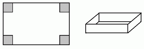
One of my department colleagues recently received the College of Science Teaching Award and a teaching idea she shared during her presentation inspired me.  She is well-known for writing and assigning a wide range of projects in her classes at all levels.  During the presentation, she described the Paper Box project she gives in Calculus I.  If you cut squares of side length from each of the four corners of an sheet of paper, you can fold up the resulting tabs and join neighboring edges with tape to form a box.

As a project, the participating students were asked to construct various such boxes for a couple of different side lengths, use geometry to compute a formula for the volume in terms the length , graph that function, and use calculus to determine the length producing the box with maximum volume.  Part of the project even asked the students to fill the paper box models with rice in order to compare the volumes and experimentally verify their result.  To synthesize, the students were asked to produce a careful project report on which they were graded.

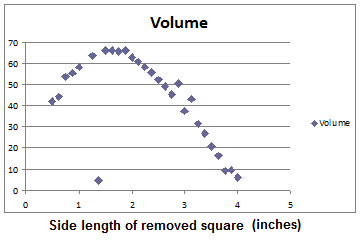
I extracted a part of this project and turned it into a class-wide activity for the second day of class.  Each of my sections has around 30 to 35 students on the first day of class.  As I took role, I distributed the numbers between 0.5 and 4 (in steps of 0.125) to each of the students. Their assignment for the second day of class was to make a box with their particular number (in inches) as the side length of the removed squares, measure its volume (in cubic inches), and then bring it to class.  At the start of the second class, the students arranged their boxes at the front of the room from small to large and then entered their volume number into a spreadsheet open on my computer.  Using the plotting features of MS Excel we created a scatter plot of the data.

The students took the opportunity to have fun with this. There were embellishments:

There were confusions:

But the end result was an honest (noisy) data set and a physical, numerical, and graphical representation of the volume of the box as a function of the length .

What I liked most about this activity was the fact that everyone was involved.  Everyone took part in building a model.  Everyone reviewed the computation of volume.  Everyone had access afterward through our course management system to the data we collected as a class.  And everyone was prepared to solve the geometry problem of finding a formula for the volume as a function of the side length of the removed squares which was the first written assignment.  By democratizing this class example instead of simply telling its story at the board, I was broadly able to implement our Learn by Doing campus philosophy.

Euclid’s Support of the Pythagorean Theorem

This quarter I’m teaching “Foundations of Geometry,” a senior level course aimed primarily at future secondary mathematics teachers.  It’s unlike any other course I’ve taught before because it has a bit of a split personality:

• one part history: examining the critiques of Euclid’s Elements and the attempts to eliminate the parallel postulate.
• one part a course in logic: discussing axiomatic systems and their properties and Hilbert’s triumphant axiomatization of geometry bringing it in line with set theory and analysis.
• one part a course in hyperbolic geometry.

We also have a course specifically on Euclidean geometry that many of these students also take, which is why the mathematical focus is on noneuclidean geometry. The course design is a learning experience for me because, although my mathematical expertise is in geometry, that expertise is in the subject geometry blossomed into during the 20th century after Hilbert’s revolution.  By bringing the foundations of the subject in line with analysis, he brought Calculus to bear on the study of geometry allowing differential and algebraic geometry, together with Klein’s Erlangen program, to subsume the classical subject.  While I know quite a bit about hyperbolic space, it is from this modern viewpoint rather than the axiomatic viewpoint of Lobachevsky.  Tentatively, I plan to close the course by connecting the old with the new, but this might be a quixotic dream.  We’ll see.

For quite some time while preparing this course, I struggled with how to begin on the first day.  I finally decided that the best hook was to begin by analyzing the most famous proposition of euclidean geometry: The Pythagorean Theorem (PT).  There is a marvelous java applet by Jim Morey which animates Euclid’s proof of the PT.  Using the applet like a PowerPoint presentation, I asked the students not to take notes but to instead listen carefully as we walked through the argument.  Once everyone was convinced, I raised the screen and asked them to help me write it down at the board.  This is actually a rather difficult task since the proof has several steps, and our prose could not be shortened by referring to numbered propositions but instead had to include reminders of what facts we were applying.  Afterwards, I asked the class to examine what we wrote and discuss the following questions in groups:

1. Does this argument convince you that the PT is true?
2. What terminology is used in the proof?
3. What facts are being applied?
4. Most importantly: where exactly is the assumption that the triangle is right used in the argument?

If you watch Morey’s applet, you may miss the answer to 4. It’s actually rather subtle.  This brought out some good discussion and I took the opportunity to highlight how a proof can be correct without necessarily being completely clear, and that good proof writing makes the use of assumptions apparent.

After this, I had them engage in a group discussion activity analyzing several different proofs of the PT culled from the list hosted at cut-the-knot.org compiled by Alexander Bogomolny.  In addition to my favorite dissection proof of the PT, a similar triangles argument, and Da Vinci’s quadrilateral argument for the PT, I slipped in a false proof to make sure that they were answering question 1 honestly.

The false argument appeared in the American Mathematical Monthly in 1896 and was later retracted.  It commits the fallacy of Affirming the Consequent, a mistake that I have seen many students make when first learning proof-writing.  This gave a nice segue into the discussion of logic.  The seminal achievement of Euclid and the Greek geometers was to take geometric thinking and recast it as a deductive science, in which the known geometric results of the time were organized to follow from a few simple assumptions.  This was the birth of the axiomatic method.

I wanted to convey in some manner what an achievement this was.  The directed graph below is what I made to do this.  The numbers of the nodes correspond to the propositions in Book I of the Elements.  Proposition 47 in Book I is the Pythagorean Theorem and is the node at the top.  The only propositions in Book I which follow solely from the axioms are Prop. 1 and Prop 4.  These are at the bottom.  The diagram shows the intervening propositions and their network of implications (there is an arrow from i to j if prop i is used in the proof of prop j), leading from 1 and 4 to the PT at 47.

One could imagine trying to find an axiomatization of geometry by starting with something complicated like the PT, finding a proof of it using certain assumptions, then proving those using simpler ones, and so on until you reach simple candidate statements for axioms. But the fact that Euclid did so in the face of such complexity of implication (perhaps not so complex by modern standards but certainly complex for 300 BCE) is really impressive to me.

A Celebratory Finish

We concluded my Linear Algebra classes with a project poster session.  In each section, there were eight groups of three to four students each.  The posters were hung on the walls around the room and throughout the hour, a member (or members) of the group had to stand by their poster to summarize and explain the project to their fellow students while the others mingled.  I brought some snacks, put some music on for background, and tried to remember to announce on regular intervals that people needed to rotate.  The mood was very upbeat and a few of my colleagues even came by to take in either the morning or afternoon sessions.  Overall, I was really impressed with the output of the students.  Many of them took real ownership of their project and explored their topics beyond the confines of the materials I gave them.  Moreover, it seemed that the students really enjoyed learning about the work of their classmates.  It was much better way to end the term than saying, “Any questions? Alright, we’re done.  See you at the final exam.”  In fact, in the morning section no one seemed to notice that we went 5 minutes past the end of class, they were too busy discussing.

This project activity seemed to work well, although there are several things I would like to tweak for next time.  In the planning stages prior to the quarter, I compiled a number of resources and materials which could be developed into projects, such as an article on the Google page rank algorithm, an article on facial recognition software which uses eigenvalues an eigenvectors, and some sections and chapters of various books discussing applications of linear algebra inside and outside of mathematics.  But I had trouble shaping these materials to fit the following criteria:

• with the relentless pace of the 10 week quarter, the project could not involve much more than something equivalent to a section or two of the textbook.
• the prerequisites for each project could not be very substantial and needed to have been covered by the 5th or 6th week of the quarter, so that they could have been absorbed in time to start reading the project materials.
• I wanted the students to choose their project based on their interest in the topic, not on its level of difficulty, so all projects had to present the same level of challenge.
• To serve the wide variety of interests among the students, I needed a fairly wide variety of topics, but no more than 8 per class.

Fortunately, Howard Anton’s book “Linear Algebra with Applications, 7th Ed.” devotes the final chapter entirely to applications, with one application (or several small applications following a theme) in each section.  Each section even begins with a list of the prerequisite materials.  For my first time including projects in my first attempt at teaching linear algebra, I decided simpler was better, and drafted eight of the 20 sections to be the backbone of the projects.  This was not the book I used for the course, but I was able to put my own copy on reserve with the library.  The topics were:

1. Computer Graphics: Explored the representation of an object as collection of reference points in 3-space stored in a matrix and its transformations such as rotation, translation, and scaling implemented by matrix operations.
2. Games of Strategy: Explored matrix methods and quadratic forms in the analysis of two-player zero-sum games.
3. Graph Theory: Explored matrix methods in computing the number of multistep connections in directed graphs.  One group also included a discussion of Dijkstra’s algorithm for computing minimal cost paths in weighted directed networks.
4. Markov Chains: Explored the principal interaction point of linear algebra with probability.  One group, in searching for an example beyond the reading, looked for a Markov chain model of the weather in southern Califonia only to replace it with a more interesting one from Ottawa, Canada. 🙂
5. Electrical Networks: This is fairly standard, exploring Kirchoff’s Laws in DC circuits.  I pushed them to also learn about the Wheatstone Bridge, a circuit at the core of what makes a volt meter work.  One group actually went into a lab on campus and built one to see how it worked, and really understand how linear algebra was being applied.
6. Constructing Curves and Surfaces through Points: This is a slick application of determinants to find the constants in standard forms of conics so that curve or surface fits a given number of data points.
7. Leonteif Economic Models:  Earned Leontif the Nobel Prize in Economics in 1973.  This particularly appealed to the economics graduate student taking my class.
8. Cubic Spline Interpolation: A nice topic from numerical analysis and graphics.  I was impressed that one group included in their presentation how cubic spline interpolation *in time* is used to smooth the appearance of motion in video games.

When I announced the project list, I had the students rank their topic choices first through eighth, with no ties, populating a row of a spreadsheet with the digits 1 to 8.  When I received their spreadsheets by email, I merged the data into a cost matrix with the students labeling the rows and the projects labeling the columns and a in that student’s row and under the project that was their choice.  Since their were 30-31 students in each class and only eight projects, I replicated and inserted each column four times to make the matrix nearly square.  Then I applied the Hungarian Algorithm to solve the assignment problem (special thanks to my wife for support here), sorting the students into groups on projects that they had ranked highly.  I found a pretty good solution, with no one receiving worse than their third choice.  Given that Cal Poly serves students living all over the southern California area, I also asked the students to send me the address from Google maps of a Starbucks or a Panera bread near where they lived.  Using a geocoding website I created a map of these locations with the hope that I could assign groups in such a way that group members would not live too far from one another.  Unfortunately, there were just too few students spread too far apart to make this work.  So, I created a way for them to interact electronically using our course management software.

For credit on the project, I broke it into three parts.  They earned 1/3 of the credit for participating in a discussion board activity for their group two weeks before the presentation and gained access to the rest of the points for the project.  They had to submit a rough draft of the poster 1 week in advance of the presentation for some quick feedback and another 1/3 of the credit.  The final presentation earned a portion of the final third of the credit depending on the quality if the presentation and how they answered my questions. This broke the project into hopefully manageable pieces and discouraged rush efforts before the deadline.

I think it worked well, but I would like to broaden the list of topics so that I can rotate them around as I teach this class again.  Overall, it was a great way to finish the term!

Web of Equivalent Statements

From the rules of arithmetic we can deduce the equivalence of various arithmetic expressions.  These equivalences are put to work in algebra to solve equations.  For example, the statement is a number such that ,” is equivalent to the statement “ is a number such that ,” which is equivalent to the statement “ is a number such that .  Since the right hand side of this last equation is equivalent to the fraction , this last statement informs us of the value of dictated by the original relationship.  Similarly, by the rules of logic we can deduce the equivalence of various propositions, and these equivalences are then put to work to prove theorems and expose relationships between different ideas.  Here, for example, is a chain of logically equivalent statements which solve a central problem in linear algebra: characterization of eigenvalues.

• “ is an eigenvalue of an matrix ,” is equivalent to
• “ is a scalar such that there is a nonzero vector for which ,” is equivalent to
• “ is a scalar such that the homogeneous system has a nontrivial solution,” is equivalent to
• “ is a scalar such that is not invertible,” is equivalent to
• “ is a scalar such that ,” is equivalent to
• “ is a root of the characteristic polynomial of “.

Perhaps the most powerful such logical tool one can find is an equivalence between between several seemingly different statements.  Those used above are part of the variety of equivalent conditions for invertibility of a square matrix.  Here are some of them, stated in a typical format.

Theorem. The following statements concerning a matrix are equivalent:

1. is invertible.
2. is row-equivalent to the identity matrix.
3. can be factored as a product of elementary matrices.
4. The system has exactly one solution.
5. The homogeneous system has only the trivial solution.
6. .

To prove such a statement in class, or in writing in the text, one usually resorts to a slick method of argument for the sake of brevity.  One establishes the equivalence of 1 and 2, then shows 2 implies 3 implies 4 implies 5 implies 6 implies 1 (or something like that) rather than proving 16 separate “if and only if” statements.  Such a reduction is efficient, but I wonder what impact it has on student understanding.  Do the students really understand the equivalences?  What is lost by not discussing the pairwise equivalence of all of them?  A mathematician reads a statement like this and generates mentally the 16 equivalent pairs of statements for use later.  But when one is first learning to reason with propositional logic this reaction is not necessarily catalyzed.

To initiate that learning process, I decided to showcase this result visually.  We had assembled various elements of the argument at prior moments in the term.  The main point of stating it in class (as in the book) at this point was to collect these equivalent results in one place.  Instead of a TFAE statement like the one above, I organized the information in a complete graph.

I pointed out to the students that a good study goal is to be able to explain in words the idea behind each link this web of equivalent ideas.  How well do you know/remember linear algebra? Can you explain each one?

Application Snippet: Enumeration of Spanning Trees.

This week in my linear algebra class, I started discussing determinants.  We defined/recalled the definition of the determinant of a matrix and then defined determinants of higher order square matrices inductively, using cofactor expansion about the first row.

Requiring the students to have( and use) a calculator capable of matrix operations has kept technology and computation parallel with theory in the class, and I jumped on the opportunity to discuss how slow the computation of determinants can be when done by this definition.  The fact that the definition is inductive means that the computation can be carried out by recursion.  But since the cofactor expansion about the first row of an involves computing determinants of submatrices, you can quickly explain why it takes more than floating point operations in general to compute a determinant.  One thing you should get from a course on sequences and series is that the factorial function grows VERY quickly.  Faster than the exponential function in fact (just in case my students forgot how fast the exponential function grows, I like to share this Abstruse Goose comic with them). Since 20! has more than 18 digits, that means computing the determinant of a matrix by the definition requires more than a billion billion computations.  To put this in perspective, the current MacBook Pros have 2.5 GHz processors, that roughly means 2.5 billion floating point operations per second.  In other words, computation of a determinant directly by the definition on a MacBook Pro would take at least 30 years!  That’s only the case!

Of course, the remedy for this is what we discuss next.  Determinants of triangular matrices are much faster to compute, simply calculate the product of the diagonal entries, and elementary row operations affect the determinant in very predictable ways.  A modification of Gaussian Elimination will convert a matrix to triangular form through row operations which only switch the sign of the determinant, or keep in the same.  So converting to triangular form by that algorithm, computing the determinant of the triangular form, and multiplying by to the number of sign changes does the trick in far fewer steps.  This is the way many calculators and other machines are programmed to compute determinants of matrices.

For this week’s application snippet, I wanted a situation where you want/need to compute the determinant of a large matrix (so we could capitalize on this breakthrough of the theory).  Although I’ve shown before how massive linear systems can arise in practice, testing their solvability by computing the determinant of their coefficient matrices when they make sense would be contrived, since Gaussian-Elimination decides that for you anyway. The determinant would be superfluous.  I decided instead to mention an application of the Matrix-Tree Theorem (originally found by Kirchoff, although there appears to be debate on this) which is one of the topics they could explore in the projects.

Wired networks of computers communicate and share information through data packets transmitted through Ethernet cables.  A broadcast announcement might come in through a web server and need to be disseminated to all of the computers on the network, in which case it travels from the server to the terminals through Ethernet switches which replicate and rebroadcast the message to their other connections.  An example (picture from Computer-Network.net) is shown below on the left.

Physical redundancy in such a network is good.  If a mouse chews through the cable between the first switch and a subswitch, the information should have another route so that the user does not loose connectivity.  On the other hand, loops in the network are bad if the switches replicate and redistribute messages because the number of data packets on loop will then amplify exponential, eventually causing hardware failure when the circuits overheat.  To remedy the latter problem, a computer program decides which switches transmit which information where so that every user receives content, but only a portion of the network free of loops is used at any one time.  An example is drawn on the network above and right. Mathematically, that portion of the network is known as a spanning tree, “spanning” because it reaches every switch and end computer, and “tree” because it resembles the network of branches in a natural tree.  The computer engineer who designs the program needs to first know how many spanning trees there are to choose from given the nature of her particular network.  Then she needs a program which determines what they are, ranks them by efficiency, etc.  But first and foremost, is the simple question, “How many spanning trees are there in my wired computer network?”  For a small network, this can be spotted by eye.  The picture below shows three spanning trees on a simple network.  A little thought convinces you that those are the only three.

As we have done before, one can encode the data of the network into a symmetric matrix (known as the adjacency matrix) by the rules described in the picture.  The new ingredient we now add is another matrix (called the degree matrix), and we work with the difference matrix .  The (simply amazing) Matrix-Tree Theorem says the following which we can verify in this example.

Why would you spend time entering a matrix and computing this massive determinant when you can spot the number of spanning trees by eye?  You wouldn’t if you were working with a small office network of computers like this.  Now it’s time to think big.  How many households and businesses are internet connected in the southern California area?  Internet service providers offer web connectivity to those millions of users everyday through network of switches, routers, and web server stations connected by thousands of fiber optic cables.  Computing the number of spanning trees in this circumstance is no task for a human.  Even entering the enormous matrix in this case is a job for a machine. But with this theorem and our use of theory to improve the computing time of determinants, we have a chance of computing the answer even for a network like this.

2010 Map of the Global Internet by Cisco Systems

Getting to know you: Diagnostic Testing

Happy New Year!

The Winter Quarter gets under way for us on Tuesday, 1/3.  I’ve been working steadily on course design and preparation for my Introduction to Linear Algebra classes.  Over the break, I read a lot about the teaching of linear algebra at the collegiate level.  For example, Carl C. Cowen, On the Centrality of Linear Algebra in the Curriculum, and Resources for Teaching Linear Algebra and Linear Algebra Gems.  Given the broad applicability of the subject, I was certain that I wanted my students to do small group projects on a variety of applications (within mathematics and without) as part of the course, so I also poured over every linear algebra textbook I could get my hands on searching for ready-to-use resources.  One thing I learned this past fall is that the analogy:

If the semester schedule is a jog then the quarter schedule is a sprint.

is an apt one.  Although both formats include the same number of hours of instruction, those hours fly by so quickly that significant advance planning is required for things like projects and (in order for them to work well) resources need to be ready for immediate deployment.  Furthermore, less can be covered in a given class because there is so much less time for the students to absorb the material (which is why orthogonality and least-squares had to be side-lined, much to my disappointment).

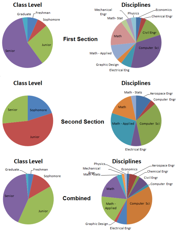
This introductory class is offered as a 2nd year course and requires a C or better in our first multivariate calculus class.  Asking around, I gained the impression that this class is typically populated by math majors.  So, I was happily designing a course and projects for sophomore mathematics majors a few weeks ago when it occurred to me to check the roster and see who was really going to be taking my classes.  Imagine my surprise when I compiled the following roster statistics.

Quite frankly, I was speechless.  I was aware, from reading the above resources, that Linear Algebra is steadily being demanded by more and more client disciplines but I certainly didn’t expect this kind of a spread.  Furthermore, the breadth of experience (judged by class level) still amazes me.  This revelation brought about a complete re-design of the projects and a different perspective on what the course should be like.  In my mind now I constantly have the question: How do I maintain challenge and interest among the more experienced students while not losing the students whom the class is supposed to be pitched for?

To get a better picture of who the students are and what they know, I decided to deploy a diagnostic test before the start of the quarter.  As an incentive, I gave a few course course points to the students for completion of the diagnostic, but their score has no impact on their grade in the course.  I looked around to see if anyone had developed a concept inventory test for Linear Algebra with no luck.  So I had to design one myself.  My goals with this test were:

1. to gauge the students experience with elementary material,
2. to determine what misconceptions they are bringing to the class,
3. to have their score accurately reflect their level of initial confusion, and
4. to have it be automatically graded.

To achieve 4, I knew I would use Blackboard’s (our course management software) testing/grading feature.  The difficulty was designing a test that would be relatively short and achieve 1, 2, and 3.

It was difficult to know where to start.  After thinking about it for a while, I decided to look up the California State K12 Mathematics Content Standards and review the linear algebra content.  Nearly all of my students were educated in southern California and the standards have been in place since December of 1997.  I chose 9 of the 11 standards to design questions around and added one more about the equations of planes in 3-space for a total of 10 questions.  Each question was multiple choice with 5 answers to choose from, one of which was a bail-out option.  For example, if the question was about determinants, the bail-out option was something like “I don’t know what a determinant is.”  After all, I would learn nothing if a student guessed among answers when they had no idea what the concept was about.  In order to meet 3, I tried to write questions that were sophisticated enough to allow me to rank the non-bailout options by level of confusion.  Since one can assign partial credit to multiple choice questions in Blackboard, their score would then give a linear scale of mastery, from unfamiliar (0 out of 4) to mastered (4 out of 4) for each topic.  In order for this to work, the incorrect non-bailout answers had to appeal to common misconceptions about the given topics.  For inspiration, I drew from the resources available from the Cornell Good Questions Project, a developing library of ConcepTest questions.

I think I managed to achieve the goals.  Of course, I won’t really know anything until the experiment plays out.  My plan is to ask the students to complete another diagnostic test at the end of the quarter on the same material, so that I can measure their individual normalized learning gain,

,

and get a sense of the impact of my class on their foundational knowledge.  This kind of thing is very popular in the physics education community for teaching introductory to courses to a broad audience, so I thought I would give it a shot here.  We’ll see how it goes.

Teaching Techniques of Integration, Part 3

This is the breakdown of class time by content for the second quarter course on analytic geometry and calculus (primarily intended for engineering students) that I am teaching this quarter.

It follows the required text: Stewart’s Calculus, which is one of the best selling textbooks on Calculus in the US and Canada at the university, college, and high school levels.  As such, this break down is probably fairly typical.

The finer breakdown of the two major categories is:

Applications of Integration	Techniques of Integration
Areas between curves	Substitution
Volumes by cross section	Integration by parts
Volumes of revolution by shells	Trigonometric Integrals
Work	Trigonometric Substitution
Average Value of a function	Partial Fractions
Arc length	Tables and Computer Algebra Systems

The main point of my previous two posts was to ask the question of whether it is time to tone down the emphasis on rote computations for computing formulas for antiderivatives in terms of elementary functions (the utility of which is to set up equations and solve practical problems) in favor of teaching alternative methods for such problem solving that apply concepts and utilize readily available electronic tools.  From the comments I received (here and elsewhere), this appears to be a rather polarizing issue.  Several readers missed my careful choice of words and responded as though I was advocating removing the “techniques of integration” pie piece completely from the curriculum.  Others championed such a move, possibly with caveats for including some of the techniques but not all.

My question is really more nuanced.  It’s about making strategic decisions on coverage in course design so as to deliver the highest quality course to the students I have now.  I’m asking: is it really of benefit to this generation of calculus students to spend 31% of a course on one particular method of problem solving?  What about the next generation?  Instead of 31% vs. 0%, should it be more like 21% vs. 10% now and maybe 10% vs. 21% ten years from now?  Of course, any such scale must be adjusted to the local audience.

Praise for emphasizing Rote Integral Computations

• Problem solving confidence builds with successful completion of such computations.
• Pencil and paper computations can have the effect of “making the theory real.”
• It feels like a payoff for years of training in algebra and trigonometry.
• Makes improper integrals of varying degrees of complexity, accessible and possible to analyze.
• Ability to successfully execute the algorithms for such computations makes you feel smart.
• Practice with such computations teaches you to pay attention to details.
• Many integrals that arise in the application of calculus (like can be calculated using well practiced techniques faster than they can be manually entered and evaluated by computer.
• Develops the ability to re-derive and verify integral table entries and formulas that are available for reference (especially those available from unrefereed sources).

Criticism for emphasizing Rote Integral Computations

• Problem solving confidence is stifled with repeated failure at execution of such computations.
• Emphasis on computations of this sort can make concepts opaque.  How many students think that the definition of is the symbols ?
• This is sometimes offered as the main goal for learning algebra and trigonometry.
• It substantiates the belief that is meaningless/worthless unless you can find a formula for a so that you can write down .
• Inability to execute such computations can make you feel not smart.  How many students do we lose in calculus courses because they have difficulty completing the algebraic/trigonometric aspects of such computations?
• Many integrals that arise in the application of calculus (like from the great fuel tank problem) can not be calculated using well practiced techniques faster than they can be manually entered and evaluated by a computer.

There are clearly important benefits and drawbacks, with sound points on either side.  This debate reminds me of the Laffer Curve from economics.  Suppose that you could determine a country’s production from its income tax rate.  If you believe such a function exists and is differentiable, then the curve might look like this:

where the horizontal axis is the tax rate and the vertical axis is production. Indeed, if the government collects no taxes, there is no revenue for infrastructure to support trade (roads, water treatment, currency, etc) and thus no production.  Likewise, if the government taxes at a rate of 100%, then no commerce can be done, so nothing will be produced.  Yet, it is non-negative function which, by observation, we know to be positive at some rate in between, so the curve must have horizontal tangent somewhere in between (Rolle’s Theorem).  The progressive/liberal argument is that we are always at position A.  With slightly more taxation, we could provide better support of trade and increase productivity.  The conservative argument is that we are always at position B.  By cutting taxes, we could free up funds to be used more effectively by businesses to increase productivity.

In the case of our debate, however, the roles seem to be reversed.  If the horizontal axis corresponds to emphasis (percentage of class time) on rote techniques of integration in an integral calculus course and the vertical axis corresponds to production of problem solvers then the progressive and conservative standpoints are switched.  The conservative argument is that we are at position A.  If we focus more on rote techniques and pencil and paper methods we will we will be more effective in producing masters of calculus skills and therefore more effective at producing problem solvers.  The progressive argument is that we are at position B.  If we focus less on rote techniques and pencil and paper methods, the benefits are that we can spend more time training a diversity of problem solving techniques and more effectively produce problem solvers.

Personally, I think we are at position B.   I see focusing heavily on rote techniques of integration as coming at a substantial price.  There is a technological sea change occurring in world culture and I think it having the effect of shifting the peak to the left, making emphasis at B less and less effective.  By focusing heavily on mechanical calculations we are ignoring the pivotal role that conceptual understanding and analytic reasoning using readily available tools will have in the future application of calculus and the training of effective problem solvers.

Teaching Techniques of Integration

I can’t help but wonder why we spend massive amounts of time teaching people NOW how to do pencil and paper arithmetic, algebra, and differential algebra when the primary means of communication are: a) increasingly digital, and b) a plethora of computational devices are literally at our fingertips? The principle reason I see is that mathematics can be viewed as precision training for the mind.  The payoff in accomplishing that training is that you are prepared to apply it creatively if you have the additional insight required to do so, and amazingly creative people have done amazing things with that knowledge and training.  Unfortunately, we are not machines and not everyone is capable of meeting the demands of that training on the timeline established in school, for a myriad of reasons.  So, pencil and paper computations have their place, but I wonder if it is now time to shift our emphasis, providing less training on precision computation, and instead provide training in the use of computational devices guided by more conceptual understanding of mathematics to solve bigger and messier problems.   In particular, why do we still focus so heavily on “techniques of integration” in our integral calculus courses?

(Disclaimer: the following paragraph is a bit of a rant.)   “Techniques of Integration” is actually a misnomer.  Integration-as a process of producing one function from another one having certain properties-is not something one needs “techniques” to do.  It is simply a matter of definition.  If has  the right properties to guarantee that makes sense and gives a number, then it has the right properties to ensure that makes sense for each real number with and so one can define a new function from by integration, i.e, by setting whenever .  It is a totally different matter to try to find a formula for that function in terms of sums of products of compositions of other functions you know.   That’s what you need “techniques” for.    If is continuous on , then is the antiderivative of on , so it should instead be called “techniques for computing formulas for antiderivatives in terms of elementary functions.” Unfortunately, that will never stick.  It takes too long to say.  But this naming problem leads us to say ridiculous things like, “The integral can’t be done,”  or “can’t be done exactly.”  How confusing is that?  It is a mathematical theorem (due to Liouville, I think) that you cannot  express the antiderivative of in terms of other elementary functions.  That means that you can’t express the value of this integral in terms of special values of elementary functions.

(Rant over) Is it really that important NOW to know how to compute a formula for the antiderivative of a function like in terms of the other elementary functions when you can use an internet connected computer, or web-enabled mobile device, to instantly answer such a question in an order of magnitude less time than you could doing it by hand?  For example, one can type “integrate (sec(x))^3 with respect to x” into Wolfram Alpha and hit enter (try it after you try the integral by hand).  Prior to the development of computers, mathematical modeling was done with special functions because it was those functions we could compute with because we knew their properties and special values.  The NASA engineers who sent human beings to the moon had to be masters of such techniques because such problems were at hand, had to be solved, and solving them with pencil, paper, and slide rule was actually faster than numerical estimation by computational devices.  That’s far from the case now.

One reason we still spend a lot of time on “techniques of integration” in integral calculus is inertial.  For example, students in our classes with ambitions to become engineers will eventually take the state license exams and be expected to compute integrals and solve differential equations like the NASA engineers of 60’s.  Until those criteria change, the demand for this training in engineering calculus is not likely to subside.   I often worry that such focus comes at the unfortunate price of students lacking the conceptual framework to apply that knowledge creatively.

A second reason we still spend a lot of time on “techniques of integration” is that it is easy to manufacture tons of such problems that the students can work to gain practice with problem solving.  Indeed, write down a formula consisting of sums of products of compositions of the elementary functions, differentiate, simplify using relations among the functions and you have a candidate integrand for the integral to assign.

• If that formula involves a sum, the linear property of integrals will show up in the computation.
• If it involves a product, integration by parts will show up.
• If it involves a composition, a substitution will be required, etc.
• If a trig identity was applied in simplification of the derivative, that identity will arise in computation of the anti-derivative.
• If it involves an inverse sine or cosine, then a trigonometric substitution will show up in the computation of the integral.

Is this the most effective practice in problem solving?